| Oracle7 Parallel Server Concepts and Administrator's Guide | Library |
Product |
Contents |
Index |
| Oracle7 Parallel Server Concepts and Administrator's Guide | Library |
Product |
Contents |
Index |
![]()
![]()
Attention: Always bear in mind that your goal is to minimize synchronization: this will result in optimized performance.
The chapter assumes that you have made at least a first cut of your database design. To optimize your design for a parallel server, follow the methodology suggested here.
To Optimize Database Design for a Parallel Server
This company's financial application has three areas which operate on a single database:
| Table | Contents |
| ORDER_HEADER | order number, customer name and address |
| ORDER_ITEMS | products ordered, quantity, and price |
| ORGANIZATIONS | names, addresses, phone numbers of customers and suppliers |
| ACCOUNTS_PAYABLE | tracks the company's internal purchase orders and payments for supplies and services |
| BUDGET | balance sheet of the company's expenses and income |
| FORECASTS | projects future sales and records current performance |
About 500 orders are entered per day. Each order header is updated about 4 times through its lifetime (so we expect about 4 times as many updates as inserts). There are many selects, because lots of people are querying order headers--people doing sales work, financial work, shipping, tracing the status of orders, and so on.
There are about 4 items per order. Order items are never updated: an item may be deleted and another item entered.
The ORDER_HEADER table has four indexes, and each of the other tables has a primary key index only.
Budget and Forecast activity has a much lower volume than the order tables. They are read frequently, but modified infrequently. Forecasts are updated more often than Budget, and are deleted once they go into actuals.
The vast bulk of the deletes are performed as a batch job at night: this maintenance activity does not therefore need to be included in the analysis of normal functioning of the application.
| Table Name | Daily Access Volume | |||||||
| Read Access | Write Access | |||||||
| Select | Insert | Update | Delete | |||||
| Operations | I/Os | Operations | I/Os | Operations | I/Os | Operations | I/Os | |
To fill out this worksheet, you estimate the volume of operations of each type, and then calculate the number of reads and writes (I/Os) the operations will entail.
Attention: The emphasis throughout this analysis is on relative values--gross figures that describe the normal use of an application. Even if an application does not yet exist, you can nonetheless project types of users and estimate relative levels of activity. Maintenance activity on the tables is not generally relevant to this analysis.
Note that the SELECT operation involves read access, and the INSERT, UPDATE and DELETE operations involve both read and write access. These operations access not only data blocks, but also any related index blocks.
Attention: The number of I/Os generated per operation changes by table depending on the access path of the table, and the table's size. It also changes depending on the number of indexes a table has. A small index, for example, may have only a single index branch block.
For example, Figure 14 - 1 illustrates read and write access to data in a large table in which two levels of the index are not in the buffer cache and only a high level index is cached in the SGA.
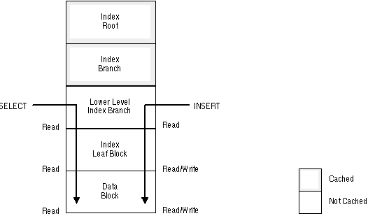 Figure 14 - 1. Number of I/Os per SELECT or INSERT Operation
In this example, assuming that you are accessing data via the primary key, a SELECT entails three I/Os:
An INSERT or DELETE statement entails at least five I/Os:
The following table shows how many I/Os are generated by each type of operation on the ORDER_HEADER table. It assumes that the ORDER_HEADER table has four indexes.
| Operation | SELECT | INSERT | UPDATE | DELETE |
| Type of Access | read | read/write | read/write | read/write |
| Number of I/Os | 3 | 14 | 7 | 14 |
Attention: Remember that you must adjust these figures depending upon the actual number of indexes and access path for each table in your database.
The following table shows how many I/Os are generated per operation for each of the other tables in the case study, assuming that each of them has a primary key index only.
| Operation | SELECT | INSERT | UPDATE | DELETE |
| Type of Access | read | read/write | read/write | read/write |
| Number of I/Os | 3 | 5 | 7 | 5 |
Note: For purposes of this analysis you can disregard the fact that any changes made to the data will also generate rollback segments, entailing additional I/Os. These I/Os are instance-based, and so should not cause problems with your parallel server application.
See Also: Oracle7 Server Concepts for more information about indexes.
| Table Name | Daily Access Volume | |||||||
| Read Access | Write Access | |||||||
| Select | Insert | Update | Delete | |||||
| Operations | I/Os | Operations | I/Os | Operations | I/Os | Operations | I/Os | |
| ORDER_HEADER | 20,000 | 60,000 | 500 | 7,000 | 2,000 | 14,000 | 1,000 | 14,000 |
| ORDER_ITEM | 60,000 | 180,000 | 2,000 | 10,000 | 0 | 0 | 4,030 | 20,150 |
| ORGANIZATIONS | 40,000 | 120,000 | 10 | 50 | 100 | 700 | 0 | 0 |
| BUDGET | 300 | 900 | 1 | 5 | 2 | 14 | 0 | 0 |
| FORECASTS | 500 | 1,500 | 1 | 5 | 10 | 70 | 2 | 10 |
| ACCOUNTS_PAYABLE | 230 | 690 | 50 | 250 | 20 | 140 | 0 | 0 |
The following conclusions can be drawn from this table:
Attention: For read-only tables, you do not need to analyze transaction volume by user type.
Use worksheets like this:
| Table Name: | |||||||||
| Type of User | No.Users | Daily Transaction Volume | |||||||
| Read Access | Write Access | ||||||||
| Select | Insert | Update | Delete | ||||||
| Operations | I/Os | Operations | I/Os | Operations | I/Os | Operations | I/Os | ||
Begin by estimating the volume of transactions by each type of user, and then calculate the number of I/Os entailed.
| Table Name: ORDER_HEADER | |||||||||
| Type of User | No.Users | Daily Transaction Volume | |||||||
| Read Access | Write Access | ||||||||
| Select | Insert | Update | Delete | ||||||
| Operations | I/Os | Operations | I/Os | Operations | I/Os | Operations | I/Os | ||
| OE clerk | 25 | 5,000 | 15,000 | 500 | 7,000 | 0 | 0 | 0 | 0 |
| AP clerk | 5 | 0 | 0 | 0 | 0 | 0 | 0 | 0 | 0 |
| AR clerk | 5 | 6,000 | 18,000 | 0 | 0 | 1,000 | 7,000 | 0 | 0 |
| Shipping clerk | 4 | 4,000 | 12,000 | 0 | 0 | 1,000 | 7,000 | 0 | 0 |
| Sales manager | 2 | 3,000 | 9,000 | 0 | 0 | 0 | 0 | 0 | 0 |
| Financial analyst | 2 | 2,000 | 6,000 | 0 | 0 | 0 | 0 | 0 | 0 |
The following conclusions can be drawn from this table:
Furthermore, the application developers realize that sales managers normally access data for the current month, whereas financial analysts access historical data.
| Table Name: ORDER_ITEMS | |||||||||
| Type of User | No.Users | Daily Transaction Volume | |||||||
| Read Access | Write Access | ||||||||
| Select | Insert | Update | Delete | ||||||
| Operations | I/Os | Operations | I/Os | Operations | I/Os | Operations | I/Os | ||
| OE clerk | 25 | 15,000 | 45,000 | 2,000 | 10,000 | 0 | 0 | 20 | 100 |
| AP clerk | 5 | 0 | 0 | 0 | 0 | 0 | 0 | 0 | 0 |
| AR clerk | 5 | 18,000 | 54,000 | 0 | 0 | 0 | 0 | 10 | 50 |
| Shipping clerk | 4 | 12,000 | 36,000 | 0 | 0 | 0 | 0 | 0 | 0 |
| Sales manager | 2 | 9,000 | 27,000 | 0 | 0 | 0 | 0 | 0 | 0 |
| Financial analyst | 2 | 6,000 | 18,000 | 0 | 0 | 0 | 0 | 0 | 0 |
The following conclusions can be drawn from this table:
Note: Although this table does not have a particularly high level of write access, we have analyzed it because it contains the main operation that the AP clerks perform.
| Table Name: ACCOUNTS_PAYABLE | |||||||||
| Type of User | No.Users | Daily Transaction Volume | |||||||
| Read Access | Write Access | ||||||||
| Select | Insert | Update | Delete | ||||||
| Operations | I/Os | Operations | I/Os | Operations | I/Os | Operations | I/Os | ||
| OE clerk | 25 | 0 | 0 | 0 | 0 | 0 | 0 | 0 | 0 |
| AP clerk | 5 | 200 | 600 | 50 | 250 | 20 | 140 | 0 | 0 |
| AR clerk | 5 | 0 | 0 | 0 | 0 | 0 | 0 | 0 | 0 |
| Shipping clerk | 4 | 0 | 0 | 0 | 0 | 0 | 0 | 0 | 0 |
| Sales manager | 2 | 0 | 0 | 0 | 0 | 0 | 0 | 0 | 0 |
| Financial analyst | 2 | 30 | 90 | 0 | 0 | 0 | 0 | 0 | 0 |
The following conclusions can be drawn from this table:
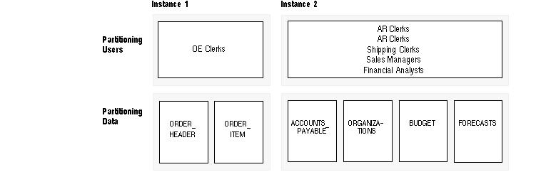 Figure 14 - 2. Case Study: Partitioning Users and Data
This system would probably be well balanced across nodes. The database intensive reporting done by financial analysts takes a good deal of system resources, whereas the transactions run by the OE clerks are relatively lightweight.
This kind of load balancing of the number of users across the system is typically useful, but not always critical. Load balancing has a lower priority for tuning than reducing contention.
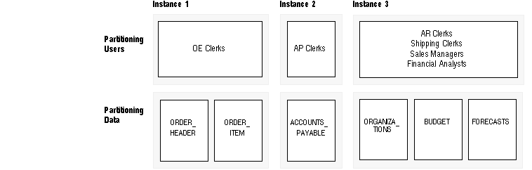 Figure 14 - 3. Case Study: Partitioning Users and Data: Design Option 1
When all users who need write access to a certain part of the data are concentrated on one node, the PCM locks will all reside on that node. In this way lock ownership will not have to go back and forth between instances.
Two design options suggest themselves, based on this analysis.
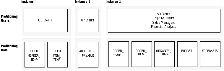 Figure 14 - 4. Case Study: Partitioning Users and Data: Design Option 2
(The problem is avoided in the Eddie Bean case study because application and data usage are partitioned.)
See Also: "Creating Free Lists for Indexes" ![[*]](jump.gif) for tips on using free lists, free list groups, and sequence numbers to avoid contention on indexes.
for tips on using free lists, free list groups, and sequence numbers to avoid contention on indexes.
"Pinpointing Lock Contention Within an Application" regarding indexes as a point of contention.
On very large tables the locking mode you use will have a strong impact on performance. If one node in exclusive mode gives 100% performance with hashed locking, one node in shared mode might give 70% of that performance with fine grain locking. The second node in shared mode would also give 70% performance. With hashed locking, the more nodes are added, the more the performance degrades. Fine grain locking is thus a more scalable solution.
You should design for worst case (hashed locking). Then, in the design or monitoring phase if you come to a situation where you have too many locks, or if you suspect false pings, you should try fine grain locking.
Begin with an analysis on the database level; you can use a worksheet like the following:
| Block Class | Relevant Parameter(s) | Use Fine Grain or Hashed Locking? |
Next, list files and database objects in a worksheet like the following, in preparation for setting GC_DB_BLOCKS. Decide which locking mode to use for each file.
| Filename | Objects Contained | Use Fine Grain or Hashed Locking? |
See Also: "Applying Fine Grain and Hashed Locking on Different Files" .
Table 9 - 4, "Initialization Parameters Which Make Block Classes Releasable," .
.
|
Prev Next |
Copyright © 1996 Oracle Corporation. All Rights Reserved. |
Library |
Product |
Contents |
Index |